A Mixed Graph Framework to Evaluate the Complementarity of Communication Tools

Authors: Leonardo Carvalho, Eduardo Bezerra, Gustavo Guedes, Laura Assis, Leonardo Lima, Rafael Barbastefano, Artur Ziviani, Fabio Porto, Eduardo Ogasawara

Federal Center for Technological Education of Rio de Janeiro (CEFET/RJ)

National Laboratory for Scientific Computing (LNCC)

Abstract: Due to the constant innovations in communications tools, several organizations are constantly evaluating the adoption of new communication tools (NCT) with respect to current ones. Especially, many organizations are interested in checking if NCT is really bringing benefits in their production process. We can state an important problem that tackles this interest as for how to identify when NCT is providing a significantly different complementary communication flow with respect to the current communication tools (CCT). This paper presents the Mixed Graph Framework (MGF) to address the problem of measuring the complementarity of a NCT in the scenario where some CCT is already established. We evaluated MGF using synthetic data that represents an enterprise social network (ESN) in the context of well-established e-mail communication tool. Our experiments observed that the MGF was able to identify whether a NCT produces significant changes in the overall communications according to some centrality measures.

Acknowledgments: The authors thank CNPq, CAPES, and FAPERJ for partially sponsoring this research.

Experimental Evaluation:

The evaluation of the proposed MGF in measuring if a NCT brings complementarity to a CCT for scenarios of Small Medium Enterprises (SME). We used synthetic data to simulate both CCT and NCT usage to explore the MGF under different group configurations and enterprise scales. Both MGF and experimental evaluation is made available at https://github.com/eogasawara/mgf.

Preprint at https://peerj.com/preprints/3114v1/

Evaluating Temporal Aggregation for Predicting the Sea Surface Temperature of the Atlantic Ocean

Authors: Rebecca Salles, Patricia Mattos, Ana-Maria Dubois Iorgulescu, Eduardo Bezerra, Leonardo Lima, Eduardo Ogasawara

Federal Center for Technological Education of Rio de Janeiro (CEFET/RJ)

Abstract: Extreme environmental events such as droughts affect millions of people all around the world. Although it is not possible to prevent this type of event, its prediction under different time horizons enables the mitigation of eventual damages caused by its occurrence. An important variable for identifying occurrences of droughts is the sea surface temperature (SST). In the Tropical Atlantic Ocean, SST data are collected and provided by the Prediction and Research Moored Array in the Tropical Atlantic (PIRATA) Project, which is an observation network composed of sensor buoys arranged in this region. Sensors of this type, and more generally Internet of Things (IoT) sensors, commonly lead to data losses that influence the quality of datasets collected for adjusting prediction models. In this paper, we explore the influence of temporal aggregation in predicting step-ahead SST considering different prediction horizons and different sizes for training data sets. We have conducted several experiments using data collected by PIRATA Project. Our results point out scenarios for training datasets and prediction horizons indicating whether or not temporal aggregated SST time series may be beneficial for prediction.

Acknowledgments: The authors thank CNPq and FAPERJ for partially sponsoring this research.

Experimental Evaluation:

The sea surface temperature (SST) data and R-functions used to perform the experimental evaluation are available in the following RData files. Furthermore, we present scripts for generating CSV files with the computed SST prediction errors and the p-values of their statistical analysis, respectively.

Prediction Errors Generation:

Experiment.RData

#Load required packages
library(TSPred)
library(DMwR)
library(hydroGOF)

#Perform the experiment using ARIMA
PerChangeBuoysExp(SelectedBuoys,testyears=1,RW=FALSE,plot=FALSE)
#Perform the experiment using Random Walk
PerChangeBuoysExp(SelectedBuoys,testyears=1,RW=TRUE,plot=FALSE)

Statistical Analysis of the Prediction Errors:

ErrorsAnalysis.RData

library(nortest)

#Perform the statistical comparative analysis of each temporal aggregation approach
PredErrorsStats <- data.frame(BuoysExpStats(ErrorsBuoysPQ))[,c(1:4,8:10)]

#Perform the statistical comparative analysis of each temporal aggregation approach against daily Random Walk SST prediction
RWPredErrorsStats <- data.frame(BuoysExpStatsRW(ErrorsBuoysPQ,ErrorsBuoysRWPQ))[,c(1:4,8:10)]

Results:

  • The results of the statistical tests performed for analysis of the SST time series in the experimental dataset: BuoysStatisticalAnalysisResults
  • ARIMA models generated in the experimental evaluation: ARIMAModels
  • The 173,040 SST prediction errors generated in the experimental evaluation: SST_PredErrors
  • The normality tests result for the prediction errors generated in the experimental evaluation: NormalityTestsResults
  • The results of the statistical tests performed for analysis and comparison of the prediction errors generated in the experimental evaluation: ComparisonStatsTestsResults


Orthographic Educational Game for Portuguese Language Countries

Authors: Paula Chaves, Luan Paschoal, Tauan Velasco, Tiago Bento Sampaio,
Julliany Brandão, Carlos Otávio Schocair, João Quadros, Talita Oliveira, Eduardo Ogasawara

Abstract

The new orthographic agreement introduces some changes in the vocabulary of the Portuguese language. Although these changes have modified a small percentage of the vocabulary words, people are struggling to adapt to some of the new orthographic rules. Aiming to mitigate this problem using a ludic approach, we developed Orthographic Educational Game (JOE). JOE focuses predominantly on the rules of accents and hyphens. The game is divided into two modes: training and playing. In the playing mode, the current level of knowledge of the player in orthography is checked and measured. In the training mode, each word comes with a hint related to the rule that is being practiced at the moment. The game was evaluated through an experiment with both undergraduates and high school students. The results indicated that more than 80\% of students enjoyed learning orthography through the game-based approach of JOE..

JOE at PlayStore

TSPred Package for R: Functions for Benchmarking Time Series Prediction

Student: Rebecca Pontes Salles (rebeccapsalles@acm.org)

Advisor: Eduardo Ogasawara (eogasawara@ieee.org)

Description: Functions for time series prediction and accuracy assessment using automatic linear modeling. The generated linear models and its yielded prediction errors can be used for benchmarking other time series prediction methods and for creating a demand for the refinement of such methods. For this purpose, benchmark data from prediction competitions may be used.

Available at CRAN: https://CRAN.R-project.org/package=TSPred

Code repository at Git-Hub: https://github.com/RebeccaSalles/TSPred

Reference manual: TSPred.pdf

Acknowledgments: The authors thank CNPq for partially sponsoring this work.

Amê: An Environment to Learn and Analyze Adversarial Search Algorithms Using Stochastic Card Games

Students: Ana Beatriz Cruz, Sabrina Seriques, and Leonardo Preuss

Advisor: Eduardo Ogasawara

Abstract:

Computer Science students are usually enthusiastic about learning Artificial Intelligence (AI) due to the possibility of developing computer games that incorporate AI behaviors. Under this scenario, Search Algorithms (SA) are a fundamental AI subject for various games. Implementing deterministic games, varying from tic-tac-toe to chess games, are common used to teach AI. Considering the perspective of game playing, however, stochastic games are usually more fun to play and are not much explored during the AI learning process. Other approaches in AI learning include developing search algorithms to compete against each other. These approaches are relevant and engaging but lack an environment that features both algorithm design and benchmarking capabilities. To address this issue, we present Amê – an environment to support the learning process and analysis of adversarial search algorithms using a stochastic card game. We have conducted a pilot experiment with Computer Science students that developed different adversarial search algorithms for Hanafuda (a traditional Japanese card game).

Data Privacy

While playing and using AME, no user data is sent or stored at AME. Only scores associated with your gameplay are sent so that you can access your ranking data.

Published paper

Amê at Google Playstore

Manual

Supporting the Learning of Evolution Theory Using an Educational Simulator

Students: Diego Vaz Caetano, Josué Dias Cardoso and Luana Guimarães Piani Ferreira
Collaborators: Raphael Abreu, João Quadros, Joel Santos
Advisors: Leonardo Lignani, Eduardo Ogasawara

Abstract

The use of simulators as educational tools aims to increase students’ engagement in classes and seems to help them to understand difficult concepts. They can be used in natural science classes as an alternative for practical or experimental approaches when the time and space scales required are not compatible with the scholar environment. Through interactive simulators, students can explore the topic under study. Discoveries are made, predictions are confirmed or refuted by subsequent simulations, enhancing the comprehension of the phenomenon. This article presents Sim-Evolution, an educational simulator to help teachers presenting Charles Darwin’s Theory of Evolution by Natural Selection (TENS). Our intention with Sim-Evolution is to enable students to practice and comprehend TENS as a process that occurs at the population level. Given that it focuses on High School level, its interface was designed to be joyful, helping to engage students. We developed Sim-Evolution focusing on three basic biological principles that structure TENS: (i) variation, (ii) heredity and (iii) selection. Also, simulation design is based on Mendelian Genetics and population genetics. However, we intended that knowledge of these areas should not be a requisite for using Sim-Evolution. Therefore, students can observe laws of evolution and the genetic properties (genotypes) by analyzing species phenotypes and surviving populations. Sim-Evolution was evaluated by High-School students in a Biology class. Experiments indicate that students could observe TENS as a population process and were able to identify the principles of variation, heredity, and selection by indirect analysis from living species phenotypes.

App

Sim-Evolution at Google Play store
User manual


Experimental Evaluation

Evaluation Procedure

Evaluation Form

Source code at GitHub


Privacy policy

We understand that user privacy must be protected and, while our application does not collect any personal information from the user or device, we are committed to transparency and therefore feel obligated to develop this Privacy Policy, the To help the user understand what data we collect, why we collect them, and what we do with them.

Information we collect and how we use it

Our application has educational purposes and was developed under the coordination of the Computer Science Departament of CEFET/RJ (http://eic.cefet-rj.br). We collect the following application information for statistical research purposes:

  • Application Name
  • Application version
  • Date / Time of application usage
  • Simulation duration time (reported in simulation time counter)
  • Type of environment used for the simulation (Forest, Savannah or Custom)
  • Types of birds selected for the beginning of the simulation
  • Types of birds existing at the close of the simulation, with their respective quantities

The information is collected and transmitted automatically at the end of each simulation when the user exits the simulation screen.

We use this information for application usage search purposes and also for possible application feature enhancements.

When this Privacy Policy applies

Our Privacy Policy applies to Sim-Evolution and its built-in features but excludes services that Google offers on Android devices.

Our Privacy Policy does not apply to services offered by other companies or individuals, including products or websites that may be displayed to the user in search results, sites that may include Sim-Evolution services or other sites with links to our services. Our Privacy Policy does not control the information practices of other companies and organizations that advertise our services and may use cookies, pixel tags, and other technologies to deliver relevant ads.

If you have any questions or concerns about our privacy policy or our practices, please contact us at gpcacefetrj@gmail.com.


STMotif-Explorer

Pattern discovery is an important task in time series mining. A particular pattern that occurs a significant number of times in a time series is called a motif. Several approaches have been developed to discover motifs in time series. However, we can observe a clear gap regarding the exploration of the spatial-time series data according to the literature review. Also, it is challenging to understand and characterize the real meaning of the motif obtained concerning the data domain, comparing different approaches and analyzing the quality of the results obtained.

We propose STMotif Explorer, a spatial-time motif analysis system that aims to interactively discover, analyze, and visualize spatial-time motifs in different domains, offering insight to users. STMotif Explorer enables users to use and implement different spatiotemporal motif detection techniques and then run this across various domains. Besides, STMotif Explorer offers the users a set of interactive resources where it is possible to visualize and analyze the discovered motifs and compare the results from different techniques. We demonstrate the features of our system with different approaches using real data.

Demonstration Video

STMotif

Spatial-Time Motifs Discovery

Authors: Heraldo Borges, Murillo Dutra,  Rafaelli~Coutinho, Fábio Perosi, Amin Bazaz,  Florent~Masseglia, Esther Pacitti, Fábio Porto, Eduardo Ogasawara
Abstract: Discovering motifs in time series data has been widely explored. Various techniques have been developed to tackle this problem. However, when it comes to spatial-time series, a clear gap can be observed according to the literature review. This paper tackles such gap by presenting an approach to discover and rank motifs in spatial-time series, denominated Combined Series Approach (CSA). CSA is based on partitioning the spatial-time series into blocks. Inside each block, subsequences of spatial-time series are combined in a way that hash-based motif discovery algorithm is applied. Motifs are validated according to both temporal and spatial constraints. Later, motifs are ranked according to their entropy, the number of occurrences, and the proximity of their occurrences. The approach was evaluated using both synthetic and seismic datasets. CSA outperforms traditional methods designed only for time series. CSA was also able to prioritize motifs that were meaningful both in the context of synthetic data and also according to seismic specialists.
Synthetic dataset:
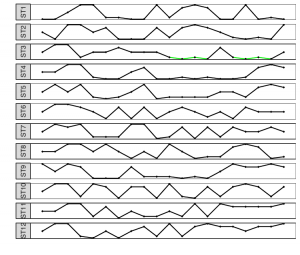
An example with 12 spatial time series. Using a traditional approach only a single motif in ST3 is found.

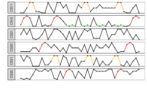
CSA approach creates some combined series from all the time series, which enables the motif discovery algorithm to discover candidate motifs that explore both spatial and time properties of the time series.

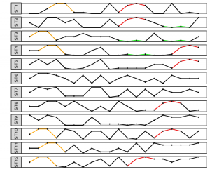
The motifs discovered are mapped into the time series and checked if they are, in fact, spatial-time motifs.

Seismic dataset:
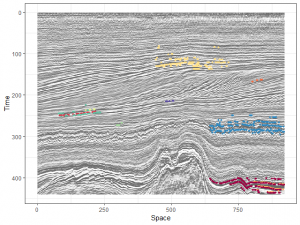
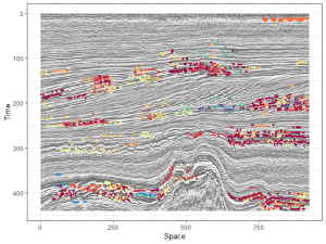
Top motifs discovered according to CSA ranking function.
Top motifs discovered according to the number of occurrences.
Code repository at Git-Hub: https://github.com/eogasawara/CSA
Acknowledgments: The authors thank CAPES, CNPq, and FAPERJ for partially sponsoring this work.

SBBD 2020 – Harbinger

Um framework para integração e análise de métodos de detecção de eventos em séries temporais

Rebecca Salles, Luciana Escobar, Lais Baroni, Roccio Zorrilla, Artur Ziviani, Vinicius Kreischer, Flavia C. Delicato, Paulo F. Pires, Luciano Maia, Rafaelli Coutinho, Laura Assis, Eduardo Ogasawara

CEFET/RJ – Centro Federal de Educação Tecnológica Celso Suckow da Fonseca
LNCC – Laboratório Nacional de Computação Científica
UFF – Universidade Federal Fluminense
Petrobras

Emails:
{rebecca.salles,luciana.vignoli,lais.baroni}@eic.cefet-rj.br
{ziviani,roccio.zorrilla,vinicius.kreischer}@lncc.br
{fdelicato,paulo.pires}@ic.uff.br, luciano.maia@petrobras.com.br
{rafaelli.coutinho,laura.assis}@cefet-rj.br, eogasawara@ieee.org

Resumo:
Ao analisar séries temporais é possível observar mudanças significativas no comportamento das observações que frequentemente caracterizam a ocorrência de eventos. Eventos se apresentam como anomalias, pontos de mudança, ou padrões frequentes. Na literatura existem diversos métodos para detecção de eventos. Entretanto, a busca por um método adequado para uma série temporal não é uma tarefa simples, principalmente considerando-se que a natureza dos eventos muitas vezes não é conhecida. Neste contexto, este trabalho apresenta Harbinger, um framework para integração e análise de métodos de detecção de eventos. O Harbinger foi avaliado em dados sintéticos e reais, onde foi possível constatar que suas funcionalidades auxiliam na escolha dos métodos e na compreensão dos eventos detectados.

Apresentação para o SBBD 2020:

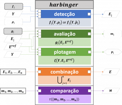
Estrutura geral de módulos

A estrutura geral do Harbinger é ilustrada na Fig. 1, sendo formada por quatro principais módulos de funcionalidade: detecção de eventos (em azul), avaliação de qualidade de detecções (em verde), combinação de resultados de detecção (em laranja), e comparação de desempenhos de detecção (em roxo). A descrição dos parâmetros de execução do Harbinger, assim como de seus artefatos produzidos é apresentada na Fig. 2. Mais informações podem ser encontradas no artigo dedicado.

Fig. 1: Diagrama geral dos módulos

diagrama_harbinger

Fig. 2: Parâmetros de execução e artefatos produzidos

Disponibilidade

O Harbinger está disponível no Github e pode ser baixado e carregado ao ambiente R com o código a seguir:

Exemplos de utilização dos métodos de detecção de eventos implementados no framework estão disponíveis em:

Utilização

Para exemplificar a utilização dos módulos do framework Harbinger vamos adotar os seguintes conjuntos de dados:

Conjuntos de dados

Série Temporal Sintética Não Estacionária (NE)

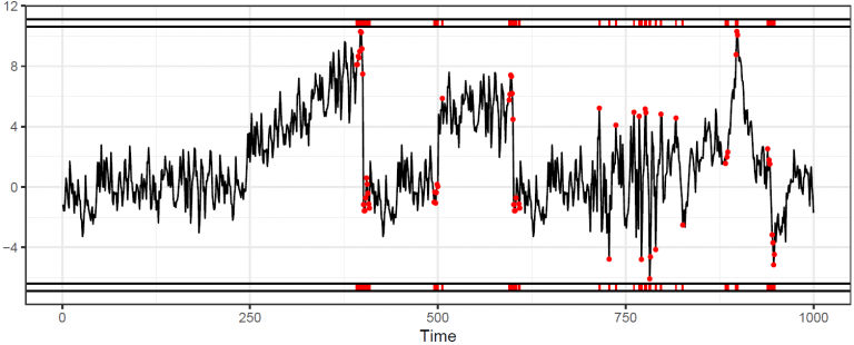
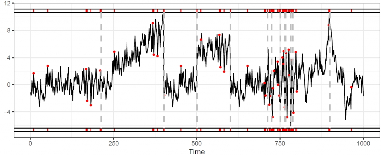
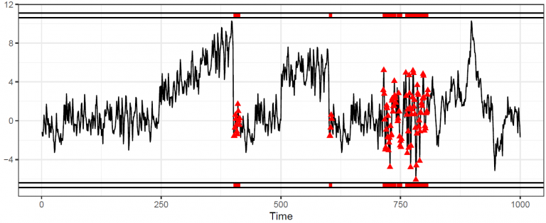
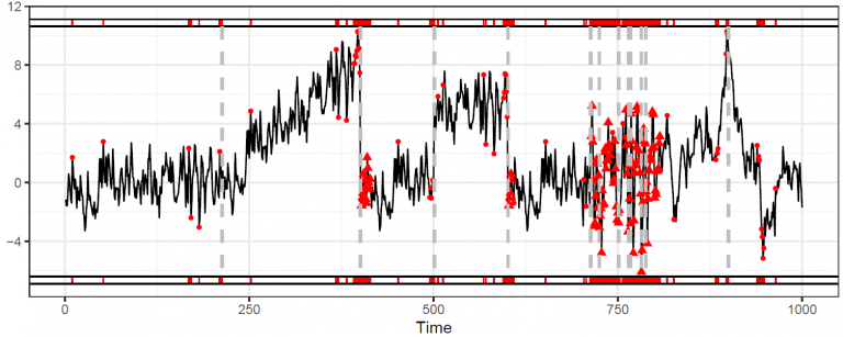
Para evidenciar as mudanças de comportamento de uma série temporal, foi desenvolvida uma série temporal sintética y com propriedades não estacionárias (NE) produzida a partir do trabalho de Salles et al. [2019]. Esta série é composta por 1000 observações (yi, i=1,…,1000) onde a subsequência <y1,…,y200> representa uma série estacionária. As demais subsequências ilustram diversas formas de não estacionariedade. Em <y201,…,y400> observa-se a estacionariedade de tendência, em <y401,…,y600> a estacionariedade de nível, em <y601,…,y800> a heteroscedasticidade, e em <y801,…,y1000> a estacionariedade por diferenciação.

Esta série temporal é construída utilizando-se o seguinte código:

> source("https://raw.githubusercontent.com/cefet-rj-dal/harbinger/master/nonstationarity_sym.r")
> nonstat_ts <- nonstationarity_sym(ts.len=200,ts.mean=0,ts.var=1)
> plot(ts(nonstat_ts),type="l",xlab="time")
Conjunto de Dados GECCO Challenge (GECCO)

Foi também utilizado para análise o conjunto de dados criado para o GECCO Challenge 2018 [Rehbach et al., 2018]. Para compor este conjunto, foram se-lecionadas 1500 observações coletadas a cada minuto contendo 72 eventos identificados. Foram coletadas 9 variáveis relacionadas à qualidade da água, das quais 5 foram selecionadas por apresentar maior variabilidade em suas observações. São elas Tp, pH, Redox, Leit e Trueb, representando a temperatura, PH, potencial Redox, condutividade elétrica e turvação, respectivamente.

Este conjunto de dados é disponibilizado pelo pacote-R EventDetectR e pode ser utilizado com o seguinte código:

> library(EventDetectR)
> gecco <- geccoIC2018Train[16500:18000,]
> plot(ts(gecco$Redox),type="l",xlab="time")

1. Módulos de detecção e combinação

A funcionalidade de detecção de eventos é responsabilidade da função chamada evtdet.

Esta função recebe como entrada os parâmetros:

  • Y: um data.frame contendo uma ou mais variáveis (séries temporais) onde a primeira variável se refere ao tempo (data ou índice sequencial).
  • ƒ: função para detecção de eventos tendo Y como entrada e um data.frame com três variáveis (time (instante/ índice de eventos), serie (nome da série correspondente) e type (tipo do evento)) como saída.
  • par: lista de parâmetros para ƒ.

A saída da função é:

  • um data.frame com três variáveis: time (instante/ índice de eventos), serie (nome da série correspondente) e type (tipo do evento).

Deste modo, a implementação da função evtdet segue o seguinte padrão:

evtdet <- function(data,func,...){
events <- do.call(func,c(list(data),list(...)))
return(events) }

Principais métodos de detecção pré-implementados:

O framework permite ao usuário a definição de métodos de detecção de eventos personalizados. Mesmo assim, Harbinger também conta com a implementação de diversos métodos de detecção de eventos. Os principais métodos implementados são descritos em seu artigo dedicado [].

Fixando as implementações dos métodos mencionados como o parâmetro ƒ da função evtdet definimos funções auxiliares para detecção de eventos. Alguns exemplos são mostrados a seguir:

  • Método AN: evtdet.an_outliers(Y,…)
  • Método CF: evtdet.changeFinder(Y,…)
  • Método GARCH: evtdet.garch_volatility_outlier(Y,…)
  • Método SCP: evtdet.seminalChangePoint(Y,…)
Exemplos de uso - Detecção de Eventos

Adaptando dados do conjunto NE para estrutura padrão do Harbinger:

> test <- data.frame(time=1:length(nonstat_ts), x=nonstat_ts)

Detecção com o método AN:

#====== Adaptive Normalization Outliers ======
#Detect
> events_an <- evtdet.an_outliers(test,w=20,alpha=1.5)
#Plot
> print(evtplot(test,events_an,reference))

Detecção com o método CF:

#====== ChangeFinder (2005) ======
#Auxiliary model definition
ARIMA <- function(data) forecast::auto.arima(data)
#Detect
> events_cf <- evtdet.changeFinder(test,mdl=ARIMA,m=5)
#Plot
> print(evtplot(test,events_cf, reference, mark.cp=TRUE))

Detecção com o método GARCH:

#====== Garch Volatility Outliers ======
#Garch specs
> garch11 <-
rugarch::ugarchspec(
    variance.model = list(model = "sGARCH", garchOrder = c(1, 1)),        mean.model = list(armaOrder = c(1, 1), include.mean = TRUE),          distribution.model = "norm")
#Detect
> events_garch <-evtdet.garch_volatility_outlier(test,spec=garch11,alpha=1.5)
#Plot
> print(evtplot(test,events_garch, reference))
Exemplo de uso - Combinação de Métodos de Detecção de Eventos

Detecção de eventos a partir da combinação dos métodos AN, CF e GARCH:

#====== Combining detected events ======
#Combining detections
> an_cf_garch <- rbind(events_an, events_cf, events_garch)
#Plot
> print( evtplot( test, an_cf_garch, mark.cp=TRUE ) )

2. Módulos de avaliação e comparação

Uma vez tendo detectado eventos em uma série temporal, é necessário avaliar a qualidade desta detecção e o desempenho do método escolhido. Esta avaliação é de responsabilidade da função evaluate.

Esta função recebe como entrada os parâmetros:

  • E: retorno da função evtdet relativo a uma série temporal particular.
  • g: função para cálculo de métrica de qualidade da detecção de eventos.
  • E_ref: data.frame com o mesmo comprimento de X contendo duas variáveis: time (tempo (data ou índice sequencial)) e event (valores booleanos indicativos da real ocorrência de eventos em X)

A saída da função é:

  • Valor da métrica de qualidade calculada.

Principais métricas de qualidade pré-implementadas:

Com o objetivo de facilitar o processo de avaliação, Harbinger conta com a implementação das principais métricas utilizadas para se avaliar a qualidade da detecção de eventos. Deste modo, a chamada à função evaluate segue o seguinte padrão:

> evaluate(E, E_ref, metric="confusion_matrix")

Neste caso, para se defnir o parâmetro g basta especificar o nome da métrica dentre as seguintes opções:

  • Matriz de confusão: “confusion_matrix”
  • Acurácia: “accuracy”
  • Sensitividade: “sensitivity”
  • Especificidade: “specificity”
  • Valor preditivo positivo: “pos_pred_value”
  • Valor preditivo negativo: “neg_pred_value”
  • Precisão: “precision”
  • Revocação: “recall”
  • F1: “F1”
  • Prevalência: “prevalence”
  • Taxa de detecção: “detection_rate”
  • Prevalência de detecção: “detection_prevalence”
  • Acurácia equilibrada: “balanced_accuracy”
Exemplos de uso - Avaliação da Detecção de Eventos

Adaptando dados do conjunto GECCO para estrutura padrão do Harbinger:

> test <- subset(gecco, select=c(Time, Trueb))
> reference <- subset(train, select=c(Time, EVENT))

Detecção com o método SCP:

#====== Seminal Change Point (1999) ====== 
#Detect 
> events_scp <- evtdet.seminalChangePoint(test,w=100)

Avaliação por matriz de confusão:

> evaluate(events_scp, reference, metric="confusion_matrix")

Events
Detected TRUE FALSE
TRUE 72 114
FALSE 0 1315

Avaliação por F1:

> evaluate(events_scp, reference, metric="F1")

F1
0.5581395

Avaliação por precisão:

> evaluate(events_scp, reference, metric="precision")

Precision
0.3870968

Avaliação por revocação:

> evaluate(events_scp, reference, metric="recall")

  Recall
1
Exemplo de uso - Avaliação Visual de Eventos

A avaliação visual dos eventos detectados é de responsabilidade da função evtplot.

Esta função recebe como entrada os parâmetros:

  • Y: mesmo utlizado em evtdet.
  • E: retorno da função evtdet.
  • E_ref: mesmo utilizado em evaluate.

A saída da função é:

  • Gráfico com as observações da série temporal, assim como marcações referentes aos resultados da detecção de eventos. Marcações vermelhas indicam eventos detectados. Além disso, são marcados em azul os eventos reais em E_ref, e em verde a coincidência entre o evento detectado e o evento real.
Um exemplo de sua utilização e saída é apresentado a seguir:
#Plot 
> print(evtplot(test,events_scp, reference))
Exemplo de uso - Comparação de Métodos de Detecção de Eventos

Podemos comparar o desempenho de detecção de diversos métodos de maneira a avaliar a sua adequabilidade aos dados assim como observar oportunidades de combinação de métodos:

#Detect
> events_an <- evtdet.an_outliers(test,w=100,alpha=1.5)
> events_cf <- evtdet.changeFinder(test,mdl=ARIMA,m=5)
> events_garch <- evtdet.garch_volatility_outlier(test,spec=garch11,alpha=1.5)
> events_scp <- evtdet.seminalChangePoint(test, w=50)
#Evaluate
> sapply(list(events_an,events_cf,events_garch,events_scp),
evaluate, reference, metric="F1")

F1 F1 F1 F1
0.5088339 0.1904762 0.1438356 0.4298507

Métodos de detecção personalizados

O framework permite ao usuário a definição de métodos de detecção de eventos personalizados.

Para isso, basta implementar o método em uma função (ƒ) para detecção de eventos tendo Y como entrada e um data.frame com três variáveis (time (instante/ índice de eventos), serie (nome da série correspondente) e type (tipo do evento)) como saída.

Um exemplo da implementação de tal função é dado a seguir. O código define uma função que identifica outliers nas observações de uma série temporal com base no primeiro e terceiro quartis e a distância interquartil:

> outliers <- function(data, alpha=1.5){

serie_name <- names(data)[-1]
names(data) <- c("time","serie")
serie <- data$serie

#===== Boxplot analysis of data ======
outliers.index <- function(data, alpha = 1.5){
org = length(data)
if (org >= 30) {
q = quantile(data)
IQR = q[4] - q[2]
lq1 = q[2] - alpha*IQR
hq3 = q[4] + alpha*IQR
cond = data < lq1 | data > hq3
index.out = which(cond)#data[cond,]
}
return (index.out)
}

#Returns index of outlier observations
index.out <- outliers.index(serie,alpha)

anomalies <- cbind.data.frame(time=data[index.out,"time"],
serie=serie_name,
type="anomaly")
names(anomalies) <- c("time","serie","type")

return(anomalies)
}

Uma vez implementado, o método pode ser integrado ao Harbinger da seguinte maneira:

> events <- evtdet(data, outliers, alpha=1.5)

Outra alternativa é criar uma função wrapper do método implementado como feito a seguir:

> evtdet.outliers <- function(data,...){

events <- evtdet(data, outlier , ...)

return(events)
}

Integração com sistemas de gerenciamento do ciclo de vida de modelos

No contexto de aprendizado de máquina, frequentemente usuários precisam lidar com o fardo de gerenciar um grande conjunto de artefatos produzidos durante o ciclo de vida de um modelo, como configurações de algoritmos, dados de entrada/saída e arquivos dos experimentos. Com isso, recentemente foram desenvolvidos sistemas para o gerenciamento do ciclo de vida dos modelos, como o ModelDB, Mistique e MLflow [Silva et al., 2019]. Harbinger se beneficia de tais sistemas para o gerenciamento de suas instâncias e registro de parâmetros de execução, métricas e artefatos produzidos. Este gerenciamento garante a proveniência e a reprodutibilidade das detecções de eventos. Além disso, o registro das aplicações de detecção e suas métricas computadas auxiliam a consulta e análise comparativa de desempenho dos métodos de detecção aplicados. Com esse objetivo, Harbinger se integra ao sistema MLflow [Zaharia et al., 2019] através da API de seu componente Tracking. As estruturas de dados dos parâmetros de execução e artefatos produzidos pelo Harbinger são uniformizadas com o objetivo de sistematizar o processo de execução de diferentes métodos, assim como facilitar o seu registro e busca no sistema.

Exemplo de uso - Integração com o MLFlow

Iremos utilizar a MLflow Tracking API para gerenciar as execuções de instâncias do Harbinger e registrar parâmetros, métricas, e artefatos (arquivos).

Para isso é preciso importar a API e executar a script de instalação com o seguinte código:

library(mlflow)
install_mlflow()

Com o código a seguir podemos detectar eventos utilizando o método AN e avaliar a qualidade da sua detecção. A execução do método e o registro de seus parâmetros, métricas de qualidade e artefatos podem ser feitos da seguinte forma:

#====== MLFlow run - Event detection ======

#Start run
> mlflow_start_run()

#Detect with Adaptive Normalization Outliers
> events_an <- evtdet.an_outliers(test, w=20, alpha=1.5)

#Log parameters
> mlflow_log_param("w", 20)
> mlflow_log_param("alpha", 1.5)

#Evaluate
> confusion_matrix <- evaluate(events_an, reference, metric="confusion_matrix")
> sensitivity <- evaluate(events_an, reference, metric="sensitivity")
> specificity <- evaluate(events_an, reference, metric="specificity")

#Log metrics
> mlflow_log_metric("sensitivity", sensitivity)
> mlflow_log_metric("specificity", specificity)

#Log artefacts
> write(confusion_matrix, file = "confusion_matrix.txt")
> mlflow_log_artifact("confusion_matrix.txt")
> write.csv(events_a, file = "events_a.csv")
> mlflow_log_artifact("events_a.csv")

#End run
> mlflow_end_run()